Vignettes

workflowr

• Summary
• Checks
• Past versions

Last updated: 2024-04-30

Checks: 7 0

Knit directory: XMAP-tutorial/

This reproducible R Markdown analysis was created with workflowr (version 1.7.0). The Checks tab describes the reproducibility checks that were applied when the results were created. The Past versions tab lists the development history.

---

R Markdown file: up-to-date

Great! Since the R Markdown file has been committed to the Git repository, you know the exact version of the code that produced these results.

Environment: empty

Great job! The global environment was empty. Objects defined in the global environment can affect the analysis in your R Markdown file in unknown ways. For reproduciblity it’s best to always run the code in an empty environment.

Seed: set.seed(20230213)

The command set.seed(20230213) was run prior to running the code in the R Markdown file. Setting a seed ensures that any results that rely on randomness, e.g. subsampling or permutations, are reproducible.

Session information: recorded

Great job! Recording the operating system, R version, and package versions is critical for reproducibility.

Cache: none

Nice! There were no cached chunks for this analysis, so you can be confident that you successfully produced the results during this run.

File paths: relative

Great job! Using relative paths to the files within your workflowr project makes it easier to run your code on other machines.

Repository version: 36aec62

Great! You are using Git for version control. Tracking code development and connecting the code version to the results is critical for reproducibility.

The results in this page were generated with repository version 36aec62. See the Past versions tab to see a history of the changes made to the R Markdown and HTML files.

Note that you need to be careful to ensure that all relevant files for the analysis have been committed to Git prior to generating the results (you can use wflow_publish or wflow_git_commit). workflowr only checks the R Markdown file, but you know if there are other scripts or data files that it depends on. Below is the status of the Git repository when the results were generated:

Ignored files:
    Ignored:    .DS_Store
    Ignored:    .Rhistory
    Ignored:    .Rproj.user/
    Ignored:    data/.DS_Store

Untracked files:
    Untracked:  analysis/LDL_TGP.Rmd
    Untracked:  data/xmap_susie_LDL_TGP.RData

Unstaged changes:
    Modified:   analysis/LDL.Rmd
    Modified:   analysis/_site.yml

Note that any generated files, e.g. HTML, png, CSS, etc., are not included in this status report because it is ok for generated content to have uncommitted changes.

---

These are the previous versions of the repository in which changes were made to the R Markdown (analysis/Vignettes.Rmd) and HTML (docs/Vignettes.html) files. If you’ve configured a remote Git repository (see ?wflow_git_remote), click on the hyperlinks in the table below to view the files as they were in that past version.

File	Version	Author	Date	Message
html	36aec62	mxcai	2024-04-30	commit
html	0174f6d	mxcai	2024-04-29	add example
Rmd	6b2e672	mxcai	2024-04-29	Update Vignettes.Rmd
Rmd	6eff465	mxcai	2024-04-29	add toggle
html	6eff465	mxcai	2024-04-29	add toggle
html	ab6d949	mxcai	2023-02-15	Build site.
html	1a72356	mxcai	2023-02-14	Build site.
Rmd	91ed24b	mxcai	2023-02-14	add
html	91ed24b	mxcai	2023-02-14	add
Rmd	81bc3f6	mxcai	2023-02-13	add
html	81bc3f6	mxcai	2023-02-13	add

---

Quick start with a simulated example

We start with a simulated data set for demonstrating the usage of XMAP software. This data set comprises a locus of 500 SNPs, among which 3 are causal.

library(susieR)
library(XMAP)
data("example_data")
par(mfrow = c(1, 2))
par(mar=c(3,3,2,1))
susie_plot(zs1, "z", b = Beta_true[, 1], main = "EAS GWAS",ylab="",xlab="")
title(ylab="-log10(p)",xlab="variant",line=2)
susie_plot(zs2, "z", b = Beta_true[, 2], main = "EUR GWAS",ylab="",xlab="")
title(ylab="-log10(p)",xlab="variant",line=2)

Past versions of unnamed-chunk-1-1.png

Version	Author	Date
81bc3f6	mxcai	2023-02-13

The above manhattan plots show the p-values of GWASs in EAS and EUR with red dots representing the 3 causal SNPs.

This data set is simulated without confounding bias. For demonstration, we apply XMAP by setting \(c_1=c_2=1\) here.

fit_xmap <- XMAP(simplify2array(list(R1,R2)), cbind(zs1,zs2),
                 n=c(20000,20000), K = 5,
                 Omega = OmegaHat,
                 Sig_E = c(1,1),
                 tol = 1e-6,
                 maxIter = 200, estimate_residual_variance = F, estimate_prior_variance = T,
                 estimate_background_variance = F)

To visualize the results, we plot the PIP and credible sets obtained by XMAP

# Get credible set based on R1
cs1 <- get_CS(fit_xmap, Xcorr = R1, coverage = 0.95, min_abs_corr = 0.1)
# Get credible set based on R2
cs2 <- get_CS(fit_xmap, Xcorr = R2, coverage = 0.95, min_abs_corr = 0.1)
# Get joint credible set
cs <- cs1$cs[intersect(names(cs1$cs), names(cs2$cs))]
pip <- get_pip(fit_xmap$gamma)
plot_CS(pip, cs, Beta_true[,1], main = "XMAP")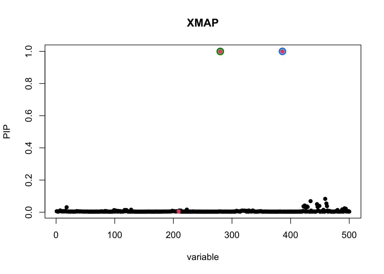

Past versions of unnamed-chunk-3-1.png

Version	Author	Date
6eff465	mxcai	2024-04-29
81bc3f6	mxcai	2023-02-13

In the above figure, the red dot is the only causal SNP, level-95% credible sets are colored circles. By combining EAS and EUR GWASs, XMAP successfully identifies two true causal signals with high confidence.

A simulated example with confounding bias

Here, we provide an example of using XMAP for correcting confounding bias in cross-population GWAS data. We simulated GWAS data with confounding effects. For demonstration, we assume that we have estimated the inflation constants \(c_1=1.636171\) and \(c_2=1.791455\), and the polygenic parameters \(\Omega\) using bi-variate LDSC (See next section for details in estimating these parameters in real GWAS data).

We first fit XMAP without correcting confounding bias by setting \(c_1=c_2=1\):

data("example_data_confound")
c1 <- 1.636171
c2 <- 1.791455
fit_xmapI <- XMAP(simplify2array(list(R1,R2)), cbind(zs1,zs2),
                  n=c(15000,20000), K = 5,
                  Omega = OmegaHat,
                  Sig_E = c(1,1),
                  tol = 1e-6,
                  maxIter = 200, estimate_residual_variance = F, estimate_prior_variance = T,
                  estimate_background_variance = F)
# Get credible set based on R1
cs1 <- get_CS(fit_xmapI, Xcorr = R1, coverage = 0.95, min_abs_corr = 0.1)
# Get credible set based on R2
cs2 <- get_CS(fit_xmapI, Xcorr = R2, coverage = 0.95, min_abs_corr = 0.1)
# Get joint credible set
cs <- cs1$cs[intersect(names(cs1$cs), names(cs2$cs))]
pip <- get_pip(fit_xmapI$gamma)
plot_CS(pip, cs, Beta_true[,1], main = "XMAP (C=I)")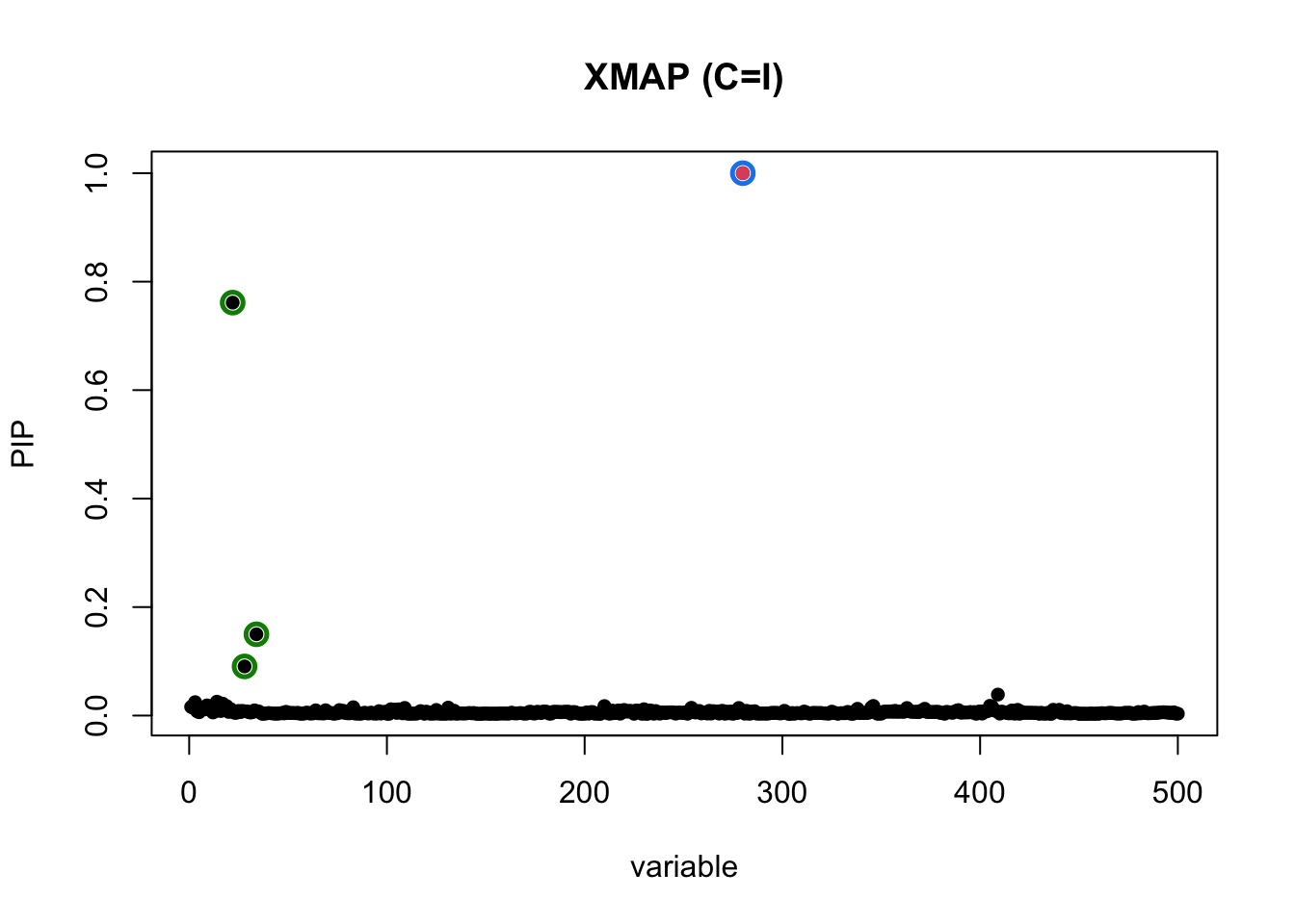

Past versions of unnamed-chunk-4-1.png

Version	Author	Date
6eff465	mxcai	2024-04-29
81bc3f6	mxcai	2023-02-13

In the above figure, the red dot is the only causal SNP, level-95% credible sets are colored circles. Without correcting for confounding bias, some null SNPs on the left region of the locus can have high PIP. These are false positives.

Now, we use the estimated LDSC intercepts to correct the confounding bias in XMAP:

c1 <- 1.636171
c2 <- 1.791455
fit_xmap <- XMAP(simplify2array(list(R1,R2)), cbind(zs1,zs2),
                 n=c(15000,20000), K = 5,
                 Omega = OmegaHat,
                 Sig_E = c(c1,c2),
                 tol = 1e-6,
                 maxIter = 200, estimate_residual_variance = F, estimate_prior_variance = T,
                 estimate_background_variance = F)
# Get credible set based on R1
cs1 <- get_CS(fit_xmap, Xcorr = R1, coverage = 0.95, min_abs_corr = 0.1)
# Get credible set based on R2
cs2 <- get_CS(fit_xmap, Xcorr = R2, coverage = 0.95, min_abs_corr = 0.1)
# Get joint credible set
cs <- cs1$cs[intersect(names(cs1$cs), names(cs2$cs))]
pip <- get_pip(fit_xmap$gamma)
plot_CS(pip, cs, Beta_true[,1], main = "XMAP")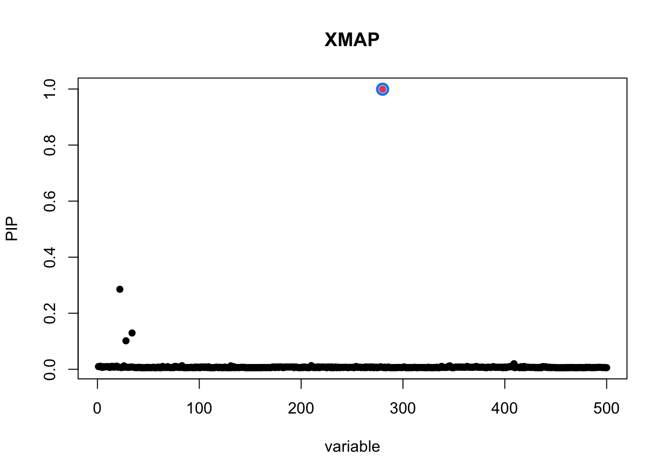

Past versions of unnamed-chunk-5-1.png

Version	Author	Date
6eff465	mxcai	2024-04-29
81bc3f6	mxcai	2023-02-13

As we can observe, XMAP effectively reduces the PIP of spurious signals and correctly excludes them from the level-95% credible sets.

A full example with LDL GWASs

In this example, we show the complete pipeline of using XMAP to identify causal SNPs by using real GWAS data. As an example, we use LDL GWASs from AFR and EUR. The files involved are:

1. GWAS summary statistics from different populations
2. LD scores estimated with samples from the analyzed populations
3. LD matrices of the target locus estimated with samples from the analyzed populations

The XMAP analysis involves two steps. We first estimate the polygenic parameters and inflation constants using GWAS summary data from the whole genome. Then we fix these parameters and use variational inference to evaluate the posteriror inclusion probability of SNPs in the target locus. In this example, we focus on the SNP rs900776 that was previously reported to be related with LDL. This SNP is located at the locus defined by base pair 20000001-23000001 in Chromosome 8. We provide the AFR and EUR LD matrices of this locus estimated from UK Biobank genotypes with the link given in the XMAP GitHub page.

library(XMAP)
library(susieR)
library(data.table)
library(Matrix)
set.seed(1)

Step 1: Estimate polygenic parameters and inflation constants

We first apply bi-variate LDCS to estimate the inflation constants and parameters of polygenic effects. We need GWASs Z-scores of the whole genome from AFR and EUR, and their LD scores as input.

We first read GWAS summary statistics and LD scores.

# read GWAS summary statistics
sumstat_EUR <- fread("/Users/cmx/Documents/Research/Project/Fine_Mapping/sumstats/LDL_allSNPs_UKBNealLab_summary_format.txt")
sumstat_AFR <- fread("/Users/cmx/Documents/Research/Project/Fine_Mapping/sumstats/LDL_AFR_GLGC_summary_format.txt")

# read LD scores
ldscore <- data.frame()
for (chr in 1:22) {
  ldscore_chr <- fread(paste0("/Users/cmx/Documents/Research/Project/Fine_Mapping/LD_ref/LD_score/LDscore_eas_brit_afr_chr", chr, ".txt"))
  ldscore <- rbind(ldscore, ldscore_chr)
  cat("CHR", chr, "\n")
}

# pre-process: remove ambiguous SNPs
idx_amb <- which(ldscore$allele1 == comple(ldscore$allele2))
ldscore <- ldscore[-idx_amb,]


# pre-process: overlap SNPs
snps <- Reduce(intersect, list(ldscore$rsid, sumstat_AFR$SNP, sumstat_EUR$SNP))
sumstat_AFR_ldsc <- sumstat_AFR[match(snps, sumstat_AFR$SNP),]
sumstat_EUR_ldsc <- sumstat_EUR[match(snps, sumstat_EUR$SNP),]
ldscore <- ldscore[match(snps, ldscore$rsid),]


# pre-process: flip alleles
z_afr <- sumstat_AFR_ldsc$beta / sumstat_AFR_ldsc$se
z_eur <- sumstat_EUR_ldsc$Z

idx_flip <- which(sumstat_AFR_ldsc$A1 != ldscore$allele1 & sumstat_AFR_ldsc$A1 != comple(ldscore$allele1))
z_afr[idx_flip] <- -z_afr[idx_flip]

idx_flip <- which(sumstat_EUR_ldsc$A1 != ldscore$allele1 & sumstat_EUR_ldsc$A1 != comple(ldscore$allele1))
z_eur[idx_flip] <- -z_eur[idx_flip]


idx1 <- which(z_afr^2 < 30 & z_eur^2 < 30)
ld_afr_w <- 1 / sapply(ldscore$AFR, function(x) max(x, 1))
ld_eur_w <- 1 / sapply(ldscore$EUR, function(x) max(x, 1))

Then we apply bi-variate LDSC to estimate polygenic and confounding parameters. The two-stage LDSC is used here.

# bi-variate LDSC: AFR-EUR
# stage 1 of LDSC: estimate intercepts
fit_step1 <- estimate_gc(data.frame(Z = z_afr[idx1], N = sumstat_AFR_ldsc$N[idx1]), data.frame(Z = z_eur[idx1], N = sumstat_EUR_ldsc$N[idx1]),
                         ldscore$AFR[idx1], ldscore$EUR[idx1], ldscore$AFR_EUR[idx1],
                         reg_w1 = ld_afr_w[idx1], reg_w2 = ld_eur_w[idx1], reg_wx = sqrt(ld_afr_w[idx1] * ld_eur_w[idx1]),
                         constrain_intercept = F)
# stage 2 of LDSC: fix intercepts and estimate slopes
fit_step2 <- estimate_gc(data.frame(Z = z_afr, N = sumstat_AFR_ldsc$N), data.frame(Z = z_eur, N = sumstat_EUR_ldsc$N),
                         ldscore$AFR, ldscore$EUR, ldscore$AFR_EUR,
                         reg_w1 = ld_afr_w, reg_w2 = ld_eur_w, reg_wx = sqrt(ld_afr_w * ld_eur_w),
                         constrain_intercept = T, fit_step1$tau1$coefs[1], fit_step1$tau2$coefs[1], fit_step1$theta$coefs[1])

We now extract the LDSC output and construct \(\hat{\Omega}\) and \(c_1\), \(c_2\) for XMAP analysis

# Assign LDSC estimates to covariance of polygenic effects
OmegaHat <- diag(c(fit_step2$tau1$coefs[2], fit_step2$tau2$coefs[2])) # AFR EUR
OmegaHat[1, 2] <- fit_step2$theta$coefs[2] # co-heritability
OmegaHat[lower.tri(OmegaHat)] <- OmegaHat[upper.tri(OmegaHat)]

c1 <- fit_step2$tau1$coefs[1] # AFR
c2 <- fit_step2$tau2$coefs[1] # EUR

Step 2: Compute posterior inclusion probability and obtain credible sets

Given the estimated polygenic parameters and inflation constants, we use variational inference to combine cross-population GWASs and evaluate PIP for SNP in the target locus. We need LD matrices and GWAS Z-scores from AFR and EUR as input.

First, we load the reference LD matrices of EUR and AFR populations estimated from UKBB samples, extract overlapped SNPs, conduct quality control, and align the effect alleles.

# read loci information
info <- fread("/Users/cmx/Documents/Research/Project/Fine_Mapping/LD_ref/LD_mat/chr8_20000001_23000001.info")

# detect allele ambiguous SNPs
idx_amb <- which(info$allele1 == comple(info$allele2))


# overlap SNPs
snps <- Reduce(intersect, list(info$rsid[-idx_amb], sumstat_AFR$SNP, sumstat_EUR$SNP))
sumstat_AFR_i <- sumstat_AFR[match(snps, sumstat_AFR$SNP),]
sumstat_EUR_i <- sumstat_EUR[match(snps, sumstat_EUR$SNP),]

# read LD matrix of AFR
R_afr <- readMM("/Users/cmx/Documents/Research/Project/Fine_Mapping/LD_ref/LD_mat/chr8_20000001_23000001_afr.mtx.gz")
R_afr <- as.matrix(R_afr + t(R_afr))
idx_afr <- match(snps, info$rsid)
R_afr <- R_afr[idx_afr, idx_afr]

# read LD matrix of EUR
R_brit <- readMM("/Users/cmx/Documents/Research/Project/Fine_Mapping/LD_ref/LD_mat/chr8_20000001_23000001_brit.mtx.gz")
R_brit <- as.matrix(R_brit + t(R_brit))
idx_brit <- match(snps, info$rsid)
R_brit <- R_brit[idx_brit, idx_brit]

info <- info[match(snps, info$rsid),]

# remove SNPs with small GWAS sample size
idx_outlier_EUR <- which(sumstat_EUR_i$N < 0.7 * median(sumstat_EUR_i$N))
idx_outlier_AFR <- which(sumstat_AFR_i$N < 0.7 * median(sumstat_AFR_i$N))

idx_outlier <- unique(c(idx_outlier_EUR, idx_outlier_AFR))

snps <- snps[-idx_outlier]
sumstat_AFR_i <- sumstat_AFR_i[-idx_outlier,]
sumstat_EUR_i <- sumstat_EUR_i[-idx_outlier,]
info <- info[-idx_outlier,]
R_afr <- R_afr[-idx_outlier, -idx_outlier]
R_brit <- R_brit[-idx_outlier, -idx_outlier]


# flip alleles
z_afr <- sumstat_AFR_i$beta / sumstat_AFR_i$se
z_eur <- sumstat_EUR_i$Z

idx_flip <- which(sumstat_AFR_i$A1 != info$allele1 & sumstat_AFR_i$A1 != comple(info$allele1))
z_afr[idx_flip] <- -z_afr[idx_flip]

idx_flip <- which(sumstat_EUR_i$A1 != info$allele1 & sumstat_EUR_i$A1 != comple(info$allele1))
z_eur[idx_flip] <- -z_eur[idx_flip]

Then, we run XMAP to obtain the PIP and credible sets

# Main XMAP analysis
xmap <- XMAP(simplify2array(list(R_brit, R_afr)), cbind(z_eur, z_afr), n=c(median(sumstat_EUR_i$N), median(sumstat_AFR_i$N)),
             K = 10, Omega = OmegaHat, Sig_E = c(c1, c2), tol = 1e-6,
             maxIter = 200, estimate_residual_variance = F, estimate_prior_variance = T,
             estimate_background_variance = F)

To visualize the results, we plot the PIP and credible sets obtained by XMAP

cs1 <- get_CS(xmap, Xcorr = R_afr, coverage = 0.9, min_abs_corr = 0.1)
cs2 <- get_CS(xmap, Xcorr = R_brit, coverage = 0.9, min_abs_corr = 0.1)
cs_xmap <- cs1$cs[intersect(names(cs1$cs), names(cs2$cs))]
pip_xmap <- get_pip(xmap$gamma)

plot_CS(pip_xmap, cs_xmap, main = "XMAP",b = (info$rsid == "rs900776"))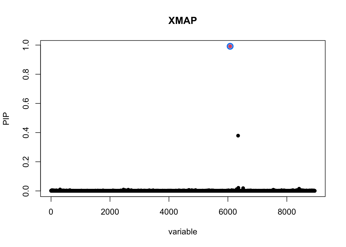

Past versions of unnamed-chunk-14-1.png

Version	Author	Date
81bc3f6	mxcai	2023-02-13

The PIP of SNP rs900776 is 0.99 as computed by XMAP.

Session information

sessionInfo()

R version 4.1.2 (2021-11-01)
Platform: aarch64-apple-darwin20 (64-bit)
Running under: macOS 13.6.3

Matrix products: default
BLAS:   /opt/homebrew/Cellar/openblas/0.3.19/lib/libopenblasp-r0.3.19.dylib
LAPACK: /Library/Frameworks/R.framework/Versions/4.1-arm64/Resources/lib/libRlapack.dylib

locale:
[1] en_US.UTF-8/en_US.UTF-8/en_US.UTF-8/C/en_US.UTF-8/en_US.UTF-8

attached base packages:
[1] stats     graphics  grDevices utils     datasets  methods   base     

other attached packages:
[1] Matrix_1.5-4.1    data.table_1.14.2 XMAP_1.0          susieR_0.12.35   

loaded via a namespace (and not attached):
 [1] tidyselect_1.2.0   xfun_0.32          bslib_0.4.0        lattice_0.20-45   
 [5] colorspace_2.0-2   vctrs_0.6.3        generics_0.1.1     htmltools_0.5.4   
 [9] yaml_2.3.5         utf8_1.2.2         rlang_1.1.1        mixsqp_0.3-43     
[13] jquerylib_0.1.4    later_1.3.0        pillar_1.9.0       glue_1.6.2        
[17] RcppZiggurat_0.1.6 matrixStats_0.61.0 lifecycle_1.0.3    plyr_1.8.6        
[21] stringr_1.4.1      munsell_0.5.0      gtable_0.3.0       workflowr_1.7.0   
[25] evaluate_0.16      knitr_1.40         fastmap_1.1.0      httpuv_1.6.5      
[29] parallel_4.1.2     irlba_2.3.5        fansi_0.5.0        Rfast_2.0.6       
[33] highr_0.9          Rcpp_1.0.10        promises_1.2.0.1   scales_1.1.1      
[37] cachem_1.0.6       jsonlite_1.8.0     fs_1.5.2           ggplot2_3.3.5     
[41] digest_0.6.29      stringi_1.7.8      dplyr_1.1.2        rprojroot_2.0.2   
[45] grid_4.1.2         cli_3.6.1          tools_4.1.2        magrittr_2.0.3    
[49] sass_0.4.2         tibble_3.2.1       crayon_1.5.1       whisker_0.4       
[53] pkgconfig_2.0.3    rmarkdown_2.16     reshape_0.8.8      rstudioapi_0.13   
[57] R6_2.5.1           git2r_0.31.0       compiler_4.1.2